Algorithms. Brute. Force

Set of sequence of unambiguous instructions for solving a problem.

Characteristics

1. Zero or more inputs: “hello world” program zero inputs
2. Definiteness: Each step should be precise and unambiguous
3. Output: At least one output
4. Effectiveness: Each step should be precise and feasible
5. Finiteness: Terminates after finite number of steps

We write algorithms in pseudo-code: A mix of natural and programming language

# Example: swap two numbers (a, b)
Algorithm swap(a,b)
Begin:
	temp = a;
	a = b;
	b = temp;
End:

We can use {} in the place of Begin: and End: The = token may also be written as := and ←

---

Fundamentals of Problem Solving

This is the framework for analyzing algorithms to solve new problems.

1. Understand the Problem
   1. Clearly define:
      1. input
      2. expected output
   2. Consider the constraints and assumptions
   3. Ensure the problem is well defined and unambiguous
2. Decide on the Computational Means
   1. Choose the appropriate model: PRAM, RAM, < TM >
   2. Evaluate the hardware and software constraints
3. Exact v/s Approximate problem solving
   1. Decide if the exact solution is feasible, or necessary
   2. Computational cost
4. Algorithmic Design Techniques
   1. Brute Force
   2. Divide and Conquer
   3. Decrease and Conquer
   4. Transform and Conquer
   5. Dynamic Programming
   6. Greedy Technique
   7. Branch and Bound
   8. Backtracking
5. Designing an Algorithm
   1. Step by step: pseudocode
   2. Algorithm follows all the characteristics
   3. Break into subroutines
6. Proving Algorithm Correctness: Works for all valid inputs
7. Analyze the algorithm
   1. Timer Complexity
   2. Space Complexity
8. Test and Debug: Test for all the cases
9. Documenting the algorithm
10. Improving and Refinement

---

Ways to Analyse

1. Time Efficiency/Complexity: how long to run as input size grows
2. Space Efficiency/Complexity: how much memory consumed as input size grows
3. Network Efficiency/Complexity
4. Hardware (Power) Efficiency/Complexity

Analyse Time and Space for

Example

Time: measure every statement as 1 unit of time Space: Frequency count of variables when algorithms are small

Algorithm swap(a,b)
Begin:
	temp <- a; (1t)
	a <- b;    (1t)
	b <- temp; (1t)
End:

• T(n) = 1+1+1 = 3 = constant
• S(n) = 1+1+1 = 3 = constant

We can represent this in the order of $O(1)$

---

Example

Notice the difference when we have a loop:

Algorithm sum(A,n)
Begin:
	s=0;
	for (i=0, i<n, i++)  // checks upto 'n+1' times, i++ 'n' times
		s = s + A[i]   // repeats upto n times
	return s;
End:

1. The dominant term is checking the condition (n+1). Consider only this
2. (2n+2) → n+1; the +2 becomes insignificant as n increases

So: T(n+1) → O(n)

---

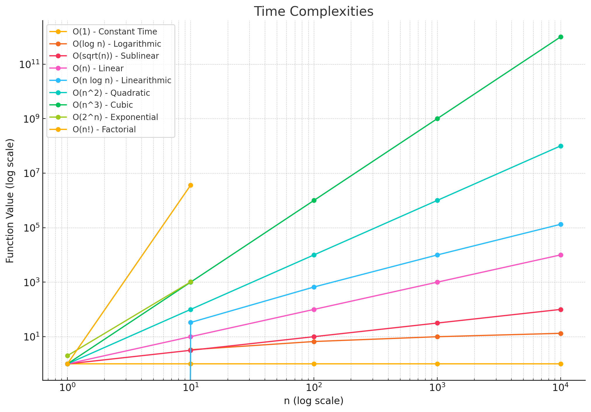
Time Complexities with Sample Values

Symbol	Name	n = 1	n = 10	n = 100	n = 1000	n = 10000
O(1)	Constant Time	1	1	1	1	1
O(log n)	Logarithmic	0	2	6	9	13
O(sqrt(n))	Sublinear	1	3	10	31	100
O(n)	Linear	1	10	100	1000	10000
O(n logn)	Linearithmic	0	33	664	9965	132877
O(n^2)	Quadratic	1	100	10000	1000000	100000000
O(n^3)	Cubic	1	1000	1000000	1000000000	1000000000000
O(2^n)	Exponential	2	1024	~1.27e30	~1.07e301	Overflow
O(n!)	Factorial	1	3.63e6	Overflow	Overflow	Overflow

---

Algorithmic Analysis Framework

1. Space Complexity

S(p) = C + SP(I)

• P is the problem
• C is the constants
• I talks about instance characteristics

2. Time Complexity

Big O, Step Count Method

3. Measuring Input Size

Efficiency of the algorithm → func

• t(n) = n
• S(n) parameters a function takes

4. Measuring Run Time

• Identify the basic operation
• Understand the concept of basic operation
• Compute total time taken for the operation

T(n) is Cop x C(n)

5. Compute the Order of Growth

Measure the performance of the algorithm in relation with input size, we must analyze for all cases of n

---

Asymptotic Notation

Asymptotic notations describe the growth of functions, often used in analyzing the time and space complexity of algorithms.

Upper Bound

Big O provides the upper bound of an algorithm’s running time, guaranteeing it won’t exceed a certain rate of growth.

Info

The function $(t(n)=O(g(n)))$ if and only if there exist constants $(C>0)$ and $(n_0\ge 0)$ such that: $[t(n)\le C\cdot g(n),\forall n\ge n_0]$

Example: $(t(n)=3n+2)$ is $(O(n))$, as $(t(n)\le 4n)$ for $(n\ge 1)$ (with $(C=4,n_0=1)$).

---

Lower Bound

Omega provides the lower bound of an algorithm’s running time, guaranteeing it takes at least a certain amount of time.

Info

The function $(t(n)=\Omega (g(n)))$ if and only if there exist constants $(C>0)$ and $(n_0\ge 0)$ such that: $[t(n)\ge C\cdot g(n),\forall n\ge n_0]$

Example: $(t(n)=3n+2)$ is $(\Omega (n))$, as $(t(n)\ge 3n)$ for $(n\ge 1)$ (with $(C=3,n_0=1)$)

---

Tight Bound

Theta provides both the upper and lower bounds, tightly bounding the growth of an algorithm’s running time.

Info

The function $(t(n)=\Theta (g(n)))$ if and only if there exist constants $(C_1,C_2>0)$ and $(n_0\ge 0)$ such that: $[C_1\cdot g(n)\le t(n)\le C_2\cdot g(n),\forall n\ge n_0]$

Example: $(t(n)=3n+2)$ is $(\Theta (n))$, as $(3n\le t(n)\le 4n)$ for $(n\ge 1)$.

---

Small o and Small ω

These notations describe stricter bounds compared to Big O and Omega.

Small $(o)$

$(t_n=o(g_n))$ means that $(t_n)$ grows asymptotically slower than $(g_n)$:

$[{\lim }_{n\to \infty }\frac{t_n}{g_n}=0]$

Small $(\omega )$

$(t_n=\omega (g_n))$ means that $(t_n)$ grows asymptotically faster than $(g_n)$:

$[{\lim }_{n\to \infty }\frac{t_n}{g_n}=\infty ]$

---

Notation	Description	Usage
$(O)$	Upper bound	Guarantees worst-case runtime
$(\Omega )$	Lower bound	Guarantees minimum runtime
$(\Theta )$	Tight bound	Represents average-case runtime
$(o)$	Strict upper bound	Stricter than Big O
$(\omega )$	Strict lower bound	Stricter than Omega

---

Analysis of Non-Recursive Algorithms

Q: Find the maximum element of an array of size ‘n’

Algorithm find_max(A, n)
Begin:
    max_element <- A[0]; 
    for i <- 1 to n-1 do:   // (n-1 times)
        if A[i] > max_element then:
            max_element <- A[i];  // (1t) larger element is found
    return max_element;
End:

1. Input size: n (size of the array).
2. Basic Operation: Comparison (comparing the current element with the maximum element).
3. C(n): The algorithm performs one comparison for each element
   1. $((u-l)+1)$
   2. $((n-1-1)+1)$
   3. $(n-1)$
4. $C(n)$=$O(n)$

Standard Formula

$C(n)={\sum }_u^{l}1=(u-l-1)$

Q: Matrix multiplication A x B

// Output Matric C = AxB
Algorithm multi(A(0..n-1, 0..n-1),B(0..n-1, 0..n-1))) {
	for (i=0; n-1) {
		for (j=0; n-1) {
			c[i, j]=(0,0)
			for (k=0; n-1) {
				c[i,j]=c[i,j] + A[i,k] * B[k,j]
			}
		}
	}
}

1. Input size: n x n
2. Basic op: Multiplication
3. $C(n)={\sum }_{i=0}^{n-1}{\sum }_{j=0}^{n-1}{\sum }_{k=0}^{n-1}1=(n^3)$

---

Analysis of Recursive Algorithms

What is the equation that relates to the algorithm??

Recurrence Relation: An equation that recursively defines a sequence. Then, we solve the recurrence relation.

1. Input size: n (size of the params).
2. Basic Operation: Same as before.
3. C(n):
   1. Substitution: Mathematical Induction, Backward Substitution
   2. Recurrence Tree
   3. Master’s

Example 1

void test(int n) {
	if (n>0) { 
		printf("%d", n);
		test(n-1);
	}
}

Recurrence Tree

           test(3)
          /      \
         3      test(2)
                /      \
               2      test(1)
                      /      \
                     1      test(0)

• $T(n)=(T(n-2)+1)$
• $T(n-1)=(T(n-1-1)+1)+1=T(n-2)+2$
• $T(n-2)+2)=(T(n-2-1)+2)+T(n-3)+3$
• $T(n-n)+n$
  • Assume $n-k=0$, $n=k$
• $T(0)+n$
• $O(n)$

Example 2

• Given: $T(n)=T(n-1)+C$

• Basecase: $T(1)=d$ ← stop the recursion

  Substitution Method:

  • $T(n)=T(n-1)+c$
  • $T(n)=(T(n-2)+c)+c=T(n)=T(n-2)+2c$
  • $T(n)=T(n-3)+3c$ so on..
  • $T(n)=T(n-k)+kc$ $n-k=1$: ← stops at base condition

$T(n)=T(n-n+1)+(n-1)c$ $T(n)=d+(n-1)c$ ← stops

Example 3

int fact(int n) {
	if (n=0) return 1 // base condition <- T(n) = 1
	else return (n * fact(n-1)) // basic op <-T(n) = 1
						// ^ for T(n-1) <- T(n-1)
}

• Given: $T(n)=1+1+T(n-1)+C$

• Basecase: $T(1)=d$ ← stop the recursion

  Substitution Method:

  • $T(n)=T(n-1)+c$
  • $T(n)=(T(n-2)+c)+c=T(n)=T(n-2)+2c$
  • $T(n)=T(n-3)+3c$ so on..
  • $T(n)=T(n-k)+kc$ $n-k=1$: ← stops at base condition Linear: $O(n)$

---

Binary Recursion

Binary recursion occurs when a recursive function makes two recursive calls during its execution. This is commonly seen in problems like computing Fibonacci numbers, binary trees, or the Towers of Hanoi.

Example: Finding the Number of Binary Digits in an Integer $n$

To find the number of binary digits (or bits) required to represent an integer $n$, we can use recursion:

Steps:

1. Base case: If $n\le 1$, it takes 1 binary digit.
2. Recursive case: Divide $n$ by 2 (integer division), and recurse.

Recursive Formula:

$$\text{BinaryDigits}(n)=\{\begin{array}{ll}1& \text{if }n\le 1,\\ 1+\text{BinaryDigits}\left(\frac{n}{2}\right)& \text{if }n>1.\end{array}$$

---

Towers of Hanoi

The Towers of Hanoi is a classic binary recursion problem where the goal is to move $n$ disks from one peg to another while adhering to the following rules:

1. Only one disk can be moved at a time.
2. No disk may be placed on top of a smaller disk.

Recursive Solution: The problem is solved recursively by breaking it into smaller subproblems:

1. Move the top $n-1$ disks to an auxiliary peg.
2. Move the largest disk directly to the destination peg.
3. Move the $n-1$ disks from the auxiliary peg to the destination peg.

TOH(n, a, b, c) {
    // IP: n (number of disks), a (source), b (auxiliary), c (destination)
    // OP: Move all disks from 'a' to 'c' in orderly fashion
 
    if (n == 1) {
        move(a, c);  // Base case: Move one disk directly
    } else {
        TOH(n - 1, a, c, b);  // Move n-1 disks to auxiliary peg
        move(a, c);           // Move the largest disk to destination peg
        TOH(n - 1, b, a, c);  // Move the n-1 disks from auxiliary peg to destination
    }
}

---

Brute Force

Ken Thompson

When in doubt use brute force!

Performance Analysis & Measurement

Performance Analysis	Performance Measurement
Involves estimation of efficiency of an algorithm theoretically.	Evaluating the exact/actual performance of an algorithm
Approach: Time and Space complexity	Approach: Measures the real execution time
Advantage: Does not depend on the system configuration, software, hardware, load.	Depends on the system load, programming language, compiler used, software and hardware.
Only an approximate efficiency calculation can be made for all the algorithm	Can give an exact estimate
Cannot get an exact estimate using a theoretical approach.	time.h or time.time()

---

Selection Sort

Scan the array, find the smallest element, swap it with the first place. Take the remaining array n→n-1 find the next smallest, and place in 2nd place; repeat until n-2

Alg selectionSort (arr[n]) {
	int smallest = -1;
	for (int i=0; i<n; i++) { // 0->n-2
		for (int j=0; j<i; j++) // i+1 -> n-1
			if (arr[j]<smallest) smallest = j
		swap(a[i], a[smallest])
	}
}

• Best: $O(n^2)$
• Worst: $O(n^2)$
• Average: $O(n^2)$

#include <stdio.h>
#include <time.h>
 
void swap(int *a, int *b)
{
	int tmp = *a;
	*a = *b;
	*b = tmp;
}
 
void display(int array[], int n)
{
	for (int i = 0; i < n; i++)
	printf("%d ", array[i]);
	printf("\n");
}
 
void selectionSort(int array[], int n)
{
	for (int i = 0; i < n - 1; i++)
	{
		int minIndex = i;
		for (int j = i + 1; j < n; j++)
		{
			if (array[j] < array[minIndex])
				minIndex = j;
		}
		swap(&array[minIndex], &array[i]);
	}
}
 
int main()
{
	int data[] = {64, 34, 25, 12, 22, 11, 90, 78, 56, 43};
	int n = sizeof(data) / sizeof(data[0]);
	printf("Original:\n");
	display(data, n);
	clock_t start = clock();
	selectionSort(data, n);
	clock_t end = clock();
	printf("Sorted:\n");
	display(data, n);
	double timeTaken = ((double)(end - start)) / CLOCKS_PER_SEC;
	printf("Time taken for sorting: %.6f seconds\n", timeTaken);
	return 0;
}

Original:
64 34 25 12 22 11 90 78 56 43 
Sorted:
11 12 22 25 34 43 56 64 78 90 
Time taken for sorting: 0.000002 seconds

---

Bubble Sort

for (i = 0; i < n - 1; i++) {
    swap = false;
    for (j = 0; j < n - 1 - i; j++) {
        if (a[j] > a[j + 1]) {
            swap(a[j], a[j + 1]);
            swap = true;
        }
    }
    if (swap == false)
        break;
}

• Best case: $O(n)$ when the array is already sorted.
• Worst case: $O(n^2)$ when the array is in reverse order (i.e., it requires the maximum number of swaps).
• Average case: $O(n^2)$ for random arrays.

---

Linear Search

int linearSearch(int arr[], int n, int ele) {
    for (int i = 0; i < n; i++) {
        if (arr[i] == ele) {
            return i;
        }
    }
    return -1;
}

• Best case: $O(1)$ when the element is found at the first position.
• Worst case: $O(n)$ when the element is not present or is at the last position.
• Average case: $O(n)$ because on average, we will have to scan through half of the array.

---

Substring Matching

Algo substring(string[], pattern[]) {
	m=len(string[])
	n=len(pattern[])
	for (i=0; i<n-m; i++) {
		for (j=0; j<m; j++) {
			if string[i+j] != pattern [j];
			break;
		}
		if (j==m) printf("pattern found at %d:", i);
}

Travelling Salesman Problem

---

Knapsack Problem

Given a knapsack, with a maximum weight $W$ There are: $n$ items, each item: weight $Wi$ and value $Vi$

Important

To determine the maximum total value that can be obtained by selecting item to place that does not exceed the total weight $W$.

Example

Item	i1	i2	i3	i4
weight	7	3	4	5
value	42	12	40	25

Total w and v

i            | total (Tw)   | total value 
----------------------------------------
i1 ----------> 7            | 42
i2 ----------> 3            | 12
i3 ----------> 4            | 40
i4 ----------> 5            | 25
i1,2 --------> 10           | 54
i1,3 --------> 11 -> X
i1,4 --------> 12 -> X
i2,3 --------> 7            | 52
i2,4 --------> 8            | 37
i3,4 --------> 9            | 65
i1,2,3 ------> 14 -> X
i1,2,4 ------> 15 -> X
i1,3,4 ------> 16 -> X
i2,3,4 ------> 12 -> X
i1,2,3,4 ----> 19 -> X

Time complexity

• included from knapsack: 1
• Excluded from knapsack: 0

For Input (n):

i) $n=1$ → 2 subsets

	0
	1

ii) $n=2$ → $2^2$ subsets

	00
	01
	10
	11

Total time complexity is

• No of subsets: $2^n$.
• Time taken to compute total weight and value for every subset: n
• Total: $2^n\ast n$
• Time: $O(n)$

---

Job Assignment

MxM	J1	J2	J3
P1	9	2	7
P2	6	4	3
P3	5	8	1

P1	P2	P3	Total
J1	J2	J3	14
J1	J3	J2	20
J2	J1	j3	19
J2	J3	J1	19
J3	J2	J1	21
J3	J1	J2	16

Time complexity

For $n=3$, 6 possibilities → $O(n+n!)$ → $O(n!)$

Too costly, instead we use:

1. Hungarian
2. Branch & Bound
3. Greedy
4. Linear Programming

---

Recurrence Relation, Dividing Functions

Decrease by one constant

int test (int n) {
	if (n<1) {
		test(n/2);
	}
}

• $T(n)$, $n=1$ and $T(n/2)+1$, $n>1$
• $T(n)$, $n=2$ and $T(\frac{n}{2^2})+2$
• $T(n)$, $n=k$ and $T(\frac{n}{2^k})+k$
• Assume: $\frac{n}{2^k}=1$ → $n=2^k$ → $k=lo{g}_2(n)$

Question

$T(\frac{n}{2}+n)$

• $1+$
• $T(n/2^2+2)+n$ +
• $T(n/2^2+1)+2n+$

$O(n)$

• $n=1$
• $T(n)=1$
• $2T(n/2)+n,n>1$

$2^{k}T(\frac{n}{2^k})+kn$

k=log n

$n\ast T(1)+logn\ast n$ ⇒ $O(nlogn)$

---

t(n)= { 1; n=2 $T(n^{0.5})+1$; n>2 }